This page illustrates how to use visualize a network model using the
tools in enaR and the network package.
Load the library of models and select one to use for this illustration.
# load data
data(enaModels)        # load library of Ecosystem Networks
names(enaModels)       # view model names
#>   [1] "Marine Coprophagy (oyster)"
#>   [2] "Lake Findley "
#>   [3] "Mirror Lake"
#>   [4] "Lake Wingra"
#>   [5] "Marion Lake"
#>   [6] "Cone Springs"
#>   [7] "Silver Springs"
#>   [8] "English Channel"
#>   [9] "Oyster Reef "
#>  [10] "Baie de Somme"
#>  [11] "Bothnian Bay"
#>  [12] "Bothnian Sea"
#>  [13] "Ythan Estuary"
#>  [14] "Sundarban Mangrove (virgin)"
#>  [15] "Sundarban Mangrove (reclaimed)"
#>  [16] "Baltic Sea"
#>  [17] "Ems Estuary"
#>  [18] "Swartkops Estuary  15"
#>  [19] "Southern Benguela Upwelling"
#>  [20] "Peruvian Upwelling"
#>  [21] "Crystal River (control)"
#>  [22] "Crystal River (thermal)"
#>  [23] "Charca de Maspalomas Lagoon"
#>  [24] "Northern Benguela Upwelling"
#>  [25] "Swartkops Estuary"
#>  [26] "Sunday Estuary"
#>  [27] "Kromme Estuary"
#>  [28] "Okefenokee Swamp"
#>  [29] "Neuse Estuary (early summer 1997)"
#>  [30] "Neuse Estuary (late summer 1997) "
#>  [31] "Neuse Estuary (early summer 1998)"
#>  [32] "Neuse Estuary (late summer 1998)"
#>  [33] "Gulf of Maine"
#>  [34] "Georges Bank"
#>  [35] "Middle Atlantic Bight"
#>  [36] "Narragansett Bay"
#>  [37] "Southern New England Bight"
#>  [38] "Chesapeake Bay"
#>  [39] "Mondego Estuary (Zostera sp. Meadows)"
#>  [40] "Mdloti Estuary (C, March 2002)"
#>  [41] "St. Marks Seagrass, site 1 (Jan.)"
#>  [42] "St. Marks Seagrass, site 1 (Feb.)"
#>  [43] "St. Marks Seagrass, site 2 (Jan.)"
#>  [44] "St. Marks Seagrass, site 2 (Feb.)"
#>  [45] "St. Marks Seagrass, site 3 (Jan.)"
#>  [46] "St. Marks Seagrass, site 4 (Feb.)"
#>  [47] "Sylt-Romo Bight (C)"
#>  [48] "Graminoids (wet)"
#>  [49] "Graminoids (dry)"
#>  [50] "Cypress (wet)"
#>  [51] "Cypress (dry)"
#>  [52] "Lake Oneida (pre-ZM)"
#>  [53] "Lake Oneida (post-ZM)"
#>  [54] "Bay of Quinte (pre-ZM)"
#>  [55] "Bay of Quinte (post-ZM)"
#>  [56] "Mangroves (wet)"
#>  [57] "Mangroves (dry)"
#>  [58] "Florida Bay (wet)"
#>  [59] "Florida Bay (dry)"
#>  [60] "Hubbard Brook (Ca)(Waide)"
#>  [61] "Hardwood Forest, NH (Ca)"
#>  [62] "Duglas Fir Forest, WA (Ca)"
#>  [63] "Duglas Fir Forest, WA (K)"
#>  [64] "Puerto Rican Rain Forest (Ca)"
#>  [65] "Puerto Rican Rain Forest (K)"
#>  [66] "Puerto Rican Rain Forest (Mg)"
#>  [67] "Puerto Rican Rain Forest (Cu)"
#>  [68] "Puerto Rican Rain Forest (Fe)"
#>  [69] "Puerto Rican Rain Forest (Mn)"
#>  [70] "Puerto Rican Rain Forest (Na)"
#>  [71] "Puerto Rican Rain Forest (Sr)"
#>  [72] "Tropical Rain Forest (N)"
#>  [73] "Neuse River Estuary (N, AVG)"
#>  [74] "Neuse River Estuary (N, Spring 1985)"
#>  [75] "Neuse River Estuary (N, Summer 1985)"
#>  [76] "Neuse River Estuary (N,  Fall 1985)"
#>  [77] "Neuse River Estuary (N, Winter 1986)"
#>  [78] "Neuse River Estuary (N, Spring 1986)"
#>  [79] "Neuse River Estuary (N, Summer 1986)"
#>  [80] "Neuse River Estuary (N, Fall 1986)"
#>  [81] "Neuse River Estuary (N, Winter 1987)"
#>  [82] "Neuse River Estuary (N, Spring 1987)"
#>  [83] "Neuse River Estuary (N, Summer 1987)"
#>  [84] "Neuse River Estuary (N, Fall 1987)"
#>  [85] "Neuse River Estuary (N, Winter 1988)"
#>  [86] "Neuse River Estuary (N, Spring 1988)"
#>  [87] "Neuse River Estuary (N, Summer 1988)"
#>  [88] "Neuse River Estuary (N, Fall 1988)"
#>  [89] "Neuse River Estuary (N, Winter 1989)"
#>  [90] "Cape Fear River Estuary (N, oligohaline)"
#>  [91] "Cape Fear River Estuary (N, polyhaline)"
#>  [92] "Lake Lanier (P) Averaged"
#>  [93] "Great Lakes (N)"
#>  [94] "Baltic Sea (N)"
#>  [95] "Chesapeake Bay (N)"
#>  [96] "Chesapeake Bay (P)"
#>  [97] "Chesapeake Bay (P, Winter)"
#>  [98] "Chesapeake Bay (P, Spring)"
#>  [99] "Chesapeake Bay (P, Summer)"
#> [100] "Chesapeake Bay (P, Fall)"
#> [101] "Sylt-Romo Bight (N)"
#> [102] "Sylt-Romo Bight (P)"
#> [103] "Beijing Urban Metabolism (C)"
#> [104] "Vienna Urban Metabolism (C)"
m <- enaModels[[9]]    # select the oyster model
Simple Plot
We can then create a simple plot of the model with the default graphics parameters as
# Set the random seed to control plot output
set.seed(2)  # this is only used to ensure our plots look the same.

# Plot network data object (uses plot.network)
plot(m)
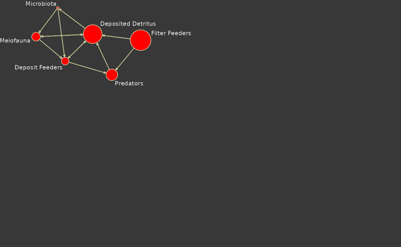
Fancy Plot
We can create a fancier plot by exerting more control on the plotting parameters. Here is an example.
  ## Set colors to use
  my.col <- c('red','yellow',rgb(204,204,153,maxColorValue=255),'grey22')
  ## Extract flow information for later use.
  F <- as.matrix(m,attrname='flow')
  ## Get indices of positive flows
  f <- which(F!=0, arr.ind=T)
  opar <- par(las=1,bg=my.col[4],xpd=TRUE,mai=c(1.02, 0.62, 0.82, 0.42))
  ## Set the random seed to control plot output
  set.seed(2)
  plot(m,
  ## Scale nodes with storage
       vertex.cex=log(m%v%'storage'),
  ## Add node labels
       label= m%v%'vertex.names',
       boxed.labels=FALSE,
       label.cex=0.65,
  ## Make rounded nodes
       vertex.sides=45,
  ## Scale arrows to flow magnitude
       edge.lwd=log10(abs(F[f])),
       edge.col=my.col[3],
       vertex.col=my.col[1],
       label.col='white',
       vertex.border = my.col[3],
       vertex.lty = 1,
       xlim=c(-4,1),ylim=c(-2,-2))